Approximate Nearest Neighbour Search

Nearest neighbour search is the question every vector database answers: given a query vector, which stored vectors are closest to it?

Done exactly, it means comparing the query against every stored vector. With a billion vectors of a thousand dimensions that is a trillion multiplications for one search — arithmetic no amount of hardware makes interactive.

Approximate search drops the guarantee. It usually returns the true nearest neighbours and occasionally misses one. What it buys for that is not a small improvement.

The measurement that matters

Here is the trade, measured rather than asserted. Forty thousand vectors in 32 dimensions, grouped into 256 clusters. A search examines only the clusters whose centres are closest to the query:

clusters examined	data scanned	exact answer found
1	0.47%	42.8%
2	0.94%	67.0%
4	1.83%	91.8%
8	3.39%	99.8%
16	6.93%	100.0%
32	13.46%	100.0%

Scanning 3.4% of the data returns the exact nearest neighbour 99.8% of the time. That is a 29× reduction in work for a 0.2% error rate — and note the shape of the curve. The first few clusters buy accuracy cheaply; past eight, the extra scanning buys nothing at all.

That knob is the entire interface of approximate search. Everything else is a question of how the candidate neighbourhoods get defined.

Why the obvious structure fails

The natural idea is to build a tree: split the space in half along one dimension, split each half again, and descend to the region containing the query. Logarithmic search, like a binary search.

It works beautifully in two or three dimensions and collapses in a hundred. The reason is worth seeing directly. Take random points and measure how much closer the nearest one is than the farthest:

dimensions	(farthest − nearest) / nearest
2	239.6
8	4.5
32	1.43
128	0.449
512	0.186

In two dimensions the farthest point is 240 times further away than the nearest. In 512 dimensions it is 1.19 times further. Everything is roughly the same distance from everything else.

A tree prunes by proving that an entire region is too far to contain the answer. When the nearest and farthest points differ by 19%, almost no region can be ruled out — so the search visits nearly every branch and performs worse than simply scanning the list, having paid for the tree as well.

This is the single most important fact about high-dimensional search, and it rules out every method that works by carving space into boxes.

What works instead

Three families survive, and they survive by not trying to prove anything.

Clustering (IVF). Group the vectors, keep one centre per group, and at query time examine only the nearest few groups. This is the method measured above. It is simple, its memory overhead is one centre per cluster, and its knob — how many groups to examine — maps directly onto the speed/accuracy curve. Its weakness is the boundary: a query sitting between two clusters may have its true neighbour in a cluster that was not examined, which is exactly what the 42.8% at one cluster reflects.

Hashing (LSH). Use hash functions designed so that nearby vectors collide. Look up the query's bucket and compare only what is in it. Attractive because accuracy is tunable by using more hash tables, and unattractive for the same reason — more tables means more copies of the index.

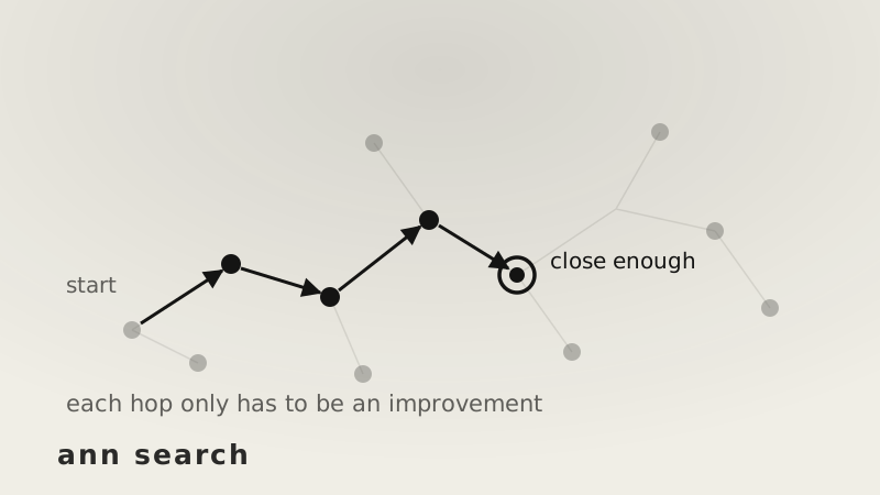
Graphs (HNSW). Build a graph where each vector links to some of its near neighbours, with a few long-range links layered on top. Search by starting somewhere and repeatedly walking to whichever neighbour is closer to the query, descending from the sparse long-range layer to the dense local one.

Graphs are what most systems use now, because the greedy walk never needs to rule a region out. It only needs each step to be an improvement, and "is this neighbour closer?" stays a meaningful question in any number of dimensions. The cost is memory for the links and a slow build — and the fact that deleting vectors from a graph is genuinely awkward, since the links that pointed at a removed node have to be repaired.

Choosing

The honest summary is short.

Graph-based indexes give the best speed at a given accuracy and cost the most memory. Clustering is cheap to build, cheap in memory, and good enough for very large collections where memory is the binding constraint — and it combines naturally with compressing the vectors themselves. Hashing is mostly of historical and theoretical interest now. Trees are for low-dimensional data, which embeddings are not.

And whichever is chosen, the parameter that decides the outcome is the same: how much of the data you are willing to look at. Measure the recall curve on your own vectors and read the flattening point off it. It will not be where the defaults put it.

What to take away

The word "approximate" undersells what is happening. This is not a degraded search.

At 3.4% of the work it returned the exact right answer in 998 cases out of 1,000. Insisting on the remaining 0.2% would have cost 29 times more — which is the kind of trade that is only difficult to make before you have measured it.