DPO

Aligning a model to human preferences traditionally takes three pieces: a model that scores responses, a critic that predicts how good a state is, and a reinforcement learning algorithm to tie them together. Four networks in memory, and a training loop with several ways to go wrong.

DPO does the same job with one training step and no reward model at all. The reason it can is a piece of algebra worth seeing.

The reward is already in there

Start from what alignment is trying to do: maximise a reward while not drifting far from the model you started with.

That problem has a known solution. The optimal policy is the reference model reweighted by the exponentiated reward:

$$\pi^*(y \mid x) = \frac{1}{Z(x)}\,\pi_{\text{ref}}(y \mid x)\,\exp\!\left(\frac{r(x,y)}{\beta}\right)$$

Now rearrange it for $r$ instead of for $\pi$:

$$r(x,y) = \beta \log \frac{\pi^*(y \mid x)}{\pi_{\text{ref}}(y \mid x)} + \beta \log Z(x)$$

Read that carefully. The reward is the log-ratio between the aligned model and the reference, plus a term that depends only on the prompt. A model that is aligned already encodes its reward function in how its probabilities differ from where it started. There is nothing left for a separate reward model to hold.

The awkward $Z(x)$ is a normaliser summing over every possible response — impossible to compute. It survives only because it is the same for every response to the same prompt, so the moment you compare two responses it cancels:

$$r(x, y_w) - r(x, y_l) = \beta\left(\log\frac{\pi(y_w)}{\pi_{\text{ref}}(y_w)} - \log\frac{\pi(y_l)}{\pi_{\text{ref}}(y_l)}\right)$$

And preference data is exactly pairwise comparisons. The one intractable term disappears precisely because of how the data is shaped.

The loss

The probability of preferring one response to another is the sigmoid of the reward gap. Maximise the likelihood of the observed preferences:

$$\mathcal{L} = -\log \sigma\!\left(\beta \left[\log\frac{\pi(y_w)}{\pi_{\text{ref}}(y_w)} - \log\frac{\pi(y_l)}{\pi_{\text{ref}}(y_l)}\right]\right)$$

Four forward passes — the trained model and the frozen reference, on the preferred and rejected responses — one loss, ordinary gradient descent. No sampling, no rollouts, no critic.

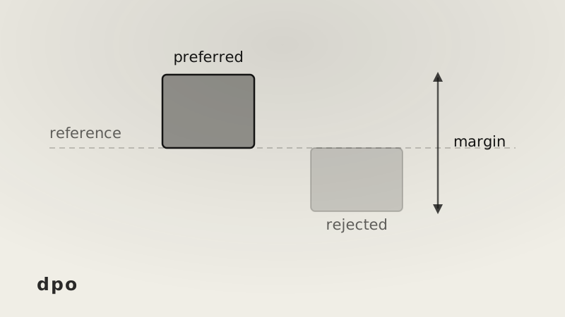
Call the bracketed quantity the margin. $\beta$ decides how hard the loss pushes on it:

margin	β = 0.1	β = 0.3	β = 0.5
−10	1.3133	3.0486	5.0067
0	0.6931	0.6931	0.6931
10	0.3133	0.0486	0.0067
20	0.1269	0.0025	0.0000

A margin of zero always costs 0.6931, which is $\log 2$ — the loss of a coin flip. Large $\beta$ makes the loss steep, so the model is pushed hard and stays near the reference only briefly; small $\beta$ keeps it gentle.

What "a difference" means in practice

Here is the part that catches people out. The loss sees the margin and nothing else.

Three ways to reach a margin of 3, all scoring identically at 0.3412:

	preferred, vs reference	rejected, vs reference
raise the preferred	×20.1	×1.00
lower the rejected	×1.00	×0.050
lower both	×0.007	×0.00034

The third row is the problem. The model has made the preferred answer about 0.7% as likely as the reference model did — and satisfied the loss perfectly, because it pushed the rejected one down even harder.

This is not hypothetical; it is a known and observed behaviour. Pushing probability mass down is easier than pushing it up, so the optimisation often takes that route, and both responses lose likelihood while the margin looks healthy. Watching the loss fall tells you nothing about it. Watching the two log-ratios separately does.

Against the reinforcement learning route

	DPO	reward model + RL
networks in memory	2 (one frozen)	4
generation during training	none	yes, constantly
kind of algorithm	supervised	reinforcement learning
stability	ordinary gradient descent	needs care
what it can learn from	the pairs you have	anything it can generate and score

The last row is the real trade. DPO learns from a fixed dataset of pairs, so it can only be as good as the pairs. The reinforcement learning route generates fresh responses from the current model, scores them, and learns from those — so it can discover behaviours nobody wrote down and keep improving as the model changes.

DPO's dataset is frozen at collection time. Once the model has moved past the responses in it, there is nothing more in there to learn.

The short version

• The optimal KL-constrained policy has a closed form, and inverting it shows the reward is the log-ratio to the reference model.
• So a language model already encodes a reward function; no separate one is needed.
• The intractable normaliser cancels in a pairwise comparison, which is exactly the shape preference data comes in.
• The loss is $-\log\sigma$ of the margin between the two log-ratios, and β sets how hard it pushes.
• Two networks instead of four, no generation during training, and plain gradient descent.
• The loss only sees the difference — both responses can drop in probability and it still looks satisfied.
• Monitor the two log-ratios separately, not just the loss.
• The trade against the RL route is learning from a fixed set of pairs instead of from what the model currently produces.