Feed-forward networks in LLMs

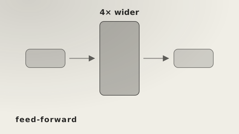
Every transformer layer has two working parts. Attention is the one that gets discussed. The other is a small, ordinary neural network applied to each token, and it holds most of the parameters.

Attention is how tokens exchange information. The feed-forward network is what each token does with that information afterwards, on its own.

Where it sits

A transformer layer runs in this order:

1. Multi-head attention
2. Add the input back, and normalise
3. Feed-forward network
4. Add the input back, and normalise

The important detail is what "each token" means here. Attention lets tokens see each other. The feed-forward network does not — it processes every token completely independently, running the same weights over each one. Tokens are handled in parallel, but no information moves between them at this stage.

What it actually does

Three steps.

$$\text{FFN}(x) = f(xW_1 + b_1)W_2 + b_2$$

First a matrix multiply that makes the vector much wider. Then an activation function. Then a second matrix multiply that brings it back to the original width.

With a model dimension of 2,048 and the usual 4× expansion:

The vector goes in at 2,048 numbers, is pushed out to 8,192, and comes back at 2,048. Same size in, same size out — but transformed.

Why widen it first

The wide middle is where the work happens.

Each of those 8,192 hidden units is looking for one thing. A unit produces a large value when its particular pattern is present in the input and roughly nothing when it is not. With 8,192 of them, the layer can check for 8,192 different patterns at once.

Picture a parcel sorting office. Parcels arrive on one belt, get spread across a hall of sorting bays — one bay per destination — and then get consolidated back onto a single outbound belt. The hall has to be wider than the belt, or there is nowhere to do the sorting. The expansion is the hall.

The contraction then compresses whatever was found back into the width the next layer expects.

The activation function

Without an activation between the two matrix multiplies, the whole thing would collapse. Two matrix multiplies in a row are just one matrix multiply, and a stack of purely linear layers is a single linear layer no matter how deep. The activation is what makes depth mean anything.

ReLU is the simplest: $\max(0, x)$. Anything negative becomes zero. That makes the hidden layer sparse — most units output nothing for any given token, and each learns to fire for its own kind of input.

GELU softens the corner. Instead of cutting negatives off abruptly it lets small negative values through, scaled down. GPT and BERT use it.

SwiGLU adds a gate. A third matrix produces a set of multipliers, and those scale the activated values elementwise — so the network learns not just what each unit computes but how much of it to let through.

That third matrix costs parameters, which is why models using SwiGLU shrink the expansion. Keeping the parameter budget fixed:

$$3 \times d \times h = 8d^2 \quad\Longrightarrow\quad h = \tfrac{8}{3}d \approx 2.67d$$

So a SwiGLU layer expands by about 2.7× rather than 4×, and ends up with the same number of weights as the two-matrix version. Implementations usually round that to a hardware-friendly multiple.

Where the knowledge lives

Attention works out relationships — which words relate to which. It does not store facts. The feed-forward network does.

Given the tallest mountain is, attention establishes that "tallest" modifies "mountain" and that the sentence is heading towards a name. The feed-forward network is what makes that name Everest. Units that learned geographic associations during training fire, and their contribution pushes the output vector towards the right answer.

That is why these layers are described as the model's memory. The patterns are distributed across thousands of units rather than stored in any single place, but the facts a model can recall live here.

Two thirds of the parameters

Count the weights in one layer, with model dimension $d$.

Attention needs four square projections — queries, keys, values, and the output — so $4d^2$.

The feed-forward network needs $d \times 4d$ going out and $4d \times d$ coming back, so $8d^2$.

At $d = 2{,}048$:

part	weights
attention	16,777,216
feed-forward	33,554,432
FFN share	66.7%

Two thirds of every layer. In a large model that is the majority of the total parameter count, sitting in the part that gets talked about least.

Splitting it into experts

Because the feed-forward network is so much of the model, it is also the part worth making conditional.

Mixture-of-experts replaces the single feed-forward network with several smaller ones and adds a router that picks which ones each token goes through. The model keeps a large total parameter count, but any individual token only activates a fraction of it. The expansion, activation and contraction inside each expert work exactly as described above.

The short version

• Every transformer layer pairs attention with a feed-forward network.
• Attention moves information between tokens; the feed-forward network transforms each token on its own.
• It expands the vector about 4×, applies an activation, and contracts it back.
• The wide middle gives room for thousands of pattern detectors; the activation is what stops the two multiplies collapsing into one.
• SwiGLU adds a gating matrix and drops the expansion to about 2.7× to keep the parameter count level.
• Roughly two thirds of a layer's weights are here, and so is most of what the model knows.