The math behind backpropagation

A neural network learns by adjusting its weights. To adjust a weight you have to know two things: which direction to move it, and how much it mattered.

Backpropagation answers both. It computes, for every weight, how much the final error would change if that weight changed slightly. Then each weight steps in whichever direction makes the error smaller.

The one rule it is built on

Everything rests on the chain rule. If $z$ depends on $y$, and $y$ depends on $x$, then:

$$\frac{dz}{dx} = \frac{dz}{dy} \times \frac{dy}{dx}$$

A network is a long chain of exactly this shape. The loss depends on the output, the output depends on the last layer, that depends on the one before it, and so on back to the input. To find how a weight near the front affects the loss at the end, you multiply the derivatives along the chain between them.

That is the whole idea. The rest is bookkeeping.

A network small enough to do by hand

Take the smallest network that still has a hidden layer: one input, one hidden neuron, one output neuron.

Each neuron does two things. First a weighted sum:

$$z = wx + b$$

Then squashes it through a sigmoid:

$$a = \sigma(z) = \frac{1}{1 + e^{-z}}$$

And the error is measured with squared loss, halved so the derivative comes out clean:

$$L = \tfrac{1}{2}(y - \hat{y})^2$$

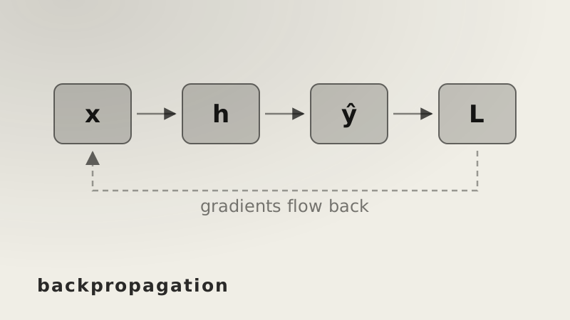
Laid out, the chain from a weight to the loss looks like this:

The forward pass

Set some numbers. Input $x = 0.9$, target $y = 0.2$, and starting parameters:

	weight	bias
hidden	$w_1 = 0.6$	$b_1 = -0.2$
output	$w_2 = -0.4$	$b_2 = 0.3$

Push the input through:

step	working	result
$z_h$	$0.6 \times 0.9 - 0.2$	0.3400
$a_h$	$\sigma(0.34)$	0.5842
$z_o$	$-0.4 \times 0.5842 + 0.3$	0.0663
$a_o$	$\sigma(0.0663)$	0.5166
$L$	$\tfrac{1}{2}(0.2 - 0.5166)^2$	0.0501

The network predicts 0.5166 where it should say 0.2. Now find out who is responsible.

The backward pass

Work right to left, one link at a time.

Start at the loss. How does it change with the prediction?

$$\frac{\partial L}{\partial a_o} = -(y - a_o) = -(0.2 - 0.5166) = 0.3166$$

Through the sigmoid. Its derivative has a convenient form, $\sigma'(z) = a(1-a)$, so no exponentials are needed a second time:

$$\frac{\partial a_o}{\partial z_o} = 0.5166 \times (1 - 0.5166) = 0.2497$$

Multiply those two and you have how the loss responds to the output neuron's pre-activation. This combined quantity is worth naming, because everything further back reuses it:

$$\delta_o = 0.3166 \times 0.2497 = 0.0791$$

The output weight. Since $z_o = w_2 a_h + b_2$, changing $w_2$ changes $z_o$ by $a_h$:

$$\frac{\partial L}{\partial w_2} = \delta_o \times a_h = 0.0791 \times 0.5842 = 0.0462$$

And the bias, whose derivative is just 1, so it inherits $\delta_o$ directly:

$$\frac{\partial L}{\partial b_2} = 0.0791$$

Keep going back. To reach the hidden neuron, carry $\delta_o$ through the output weight and the hidden sigmoid:

$$\delta_h = \delta_o \times w_2 \times a_h(1 - a_h) = 0.0791 \times (-0.4) \times 0.2429 = -0.0077$$ $$\frac{\partial L}{\partial w_1} = \delta_h \times x = -0.0077 \times 0.9 = -0.0069$$

Notice the signs differ. $\partial L/\partial w_2$ is positive, so $w_2$ must come down. $\partial L/\partial w_1$ is negative, so $w_1$ must go up. Each weight gets its own direction, and they are not the same.

That reuse of $\delta_o$ is the efficiency of the whole method. The error signal is computed once at each layer and passed backwards, rather than tracing a fresh path from every weight to the loss.

Updating the weights

Each weight moves against its gradient, scaled by a learning rate. With $\eta = 0.8$:

$$w \leftarrow w - \eta \frac{\partial L}{\partial w}$$

parameter	before	gradient	after
$w_1$	0.6	−0.0069	0.6055
$b_1$	−0.2	−0.0077	−0.1939
$w_2$	−0.4	+0.0462	−0.4369
$b_2$	0.3	+0.0791	0.2368

Run the forward pass again with those and the loss falls from 0.0501 to 0.0435, with the prediction moving from 0.5166 to 0.4951 — down towards the target of 0.2.

Repeating it

One step barely moves. Training is that step over and over:

step	loss	prediction
0	0.050110	0.5166
1	0.043536	0.4951
10	0.012865	0.3604
50	0.000322	0.2254
100	0.000010	0.2045
300	0.000000	0.2000

Same forward pass, same backward pass, same update — a few hundred times. Real networks differ by having millions of weights and many layers, but each weight is handled by exactly the arithmetic above.

The short version

• Backpropagation finds how much each weight contributed to the error.
• It works by applying the chain rule backwards through the network.
• The sigmoid's derivative is $a(1-a)$, so the forward pass supplies what the backward pass needs.
• The error signal $\delta$ is computed once per layer and reused, rather than retraced per weight.
• Each weight then steps against its own gradient, scaled by the learning rate.
• Repeat, and the loss falls.