The math behind gradient descent

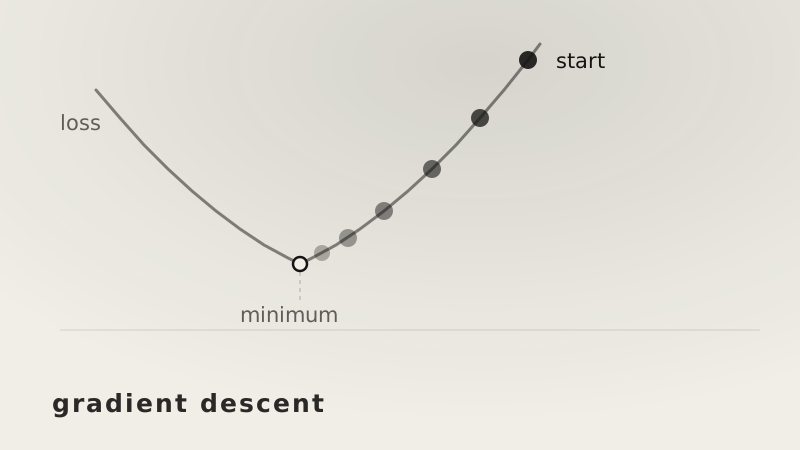
A model starts with weights that are wrong. Training is the process of nudging them until the error stops falling.

Gradient descent is how the nudging is decided. At each step it works out which direction is downhill for every weight, and moves a little that way.

Measuring how wrong it is

You cannot minimise an error you have not defined.

Say a model predicts a flat's rent as 46 and the real figure is 40. The error is 6. Square it and you get 36.

Squaring does two things. It removes the sign, so an overestimate and an underestimate both count as error rather than cancelling out. And it punishes big misses disproportionately — being wrong by 6 costs 36, but being wrong by 12 costs 144, four times as much for twice the error.

Average that over every example and you have the loss. One number saying how badly the model is doing. Everything that follows exists to make it smaller.

What the gradient tells you

The gradient of the loss with respect to a weight is its slope: how much the loss changes if that weight moves a fraction.

The sign is what matters.

• Positive gradient — increasing the weight increases the loss. So decrease it.
• Negative gradient — increasing the weight decreases the loss. So increase it.
• Zero — flat ground. Nothing to gain by moving.

The size matters too. A steep slope means the weight is far from where it should be, and a shallow one means it is close.

The update rule

Both of those facts fit in one line:

$$w \leftarrow w - \alpha \, \frac{\partial L}{\partial w}$$

The subtraction handles the direction on its own. A positive gradient gets subtracted, so the weight drops. A negative gradient subtracted is an addition, so the weight rises. Either way it moves downhill without anything checking which case it is in.

$\alpha$ is the learning rate: a small positive number setting how far to go.

Watching it run

Take a loss shaped like $f(w) = (w - 5)^2$. Its minimum is obviously at 5, which is useful — we can watch the method find something we already know.

Its gradient is $f'(w) = 2(w - 5)$. Start at $w = 12$ with $\alpha = 0.15$:

step	$w$	gradient $2(w-5)$	$w - 0.15 \times$ gradient
1	12	14	9.9
2	9.9	9.8	8.43
3	8.43	6.86	7.401
4	7.401	4.802	6.6807
5	6.6807	3.3614	6.1765

Nothing changes the step size by hand. The gradient shrinks as the weight approaches 5, so the steps shrink with it — big strides while far away, small ones near the bottom.

The step size decides everything

For this loss the whole run collapses into one line. Substituting $f'(w) = 2(w-5)$ into the update rule gives $w_{n} - 5 = (1 - 2\alpha)^{n}\,(w_0 - 5)$, so the distance to the minimum is just multiplied by $1 - 2\alpha$ every step.

That single factor explains all three behaviours:

$\alpha$	$1 - 2\alpha$	after 20 steps	what happens
0.02	0.96	$w = 8.09$	creeps — the gap shrinks 4% a step
0.15	0.70	$w = 5.0056$	converges
1.1	−1.20	$w = 273.4$	explodes

Too small and it works, just far too slowly to be useful. Too large and each step overshoots by more than it came in with, so the weight flips from side to side and the gap grows every time:

$$12 \;\rightarrow\; -3.4 \;\rightarrow\; 15.08 \;\rightarrow\; -7.096 \;\rightarrow\; 19.515$$

The condition for it to work at all is $|1 - 2\alpha| < 1$. For this loss that means $\alpha$ has to sit between 0 and 1, and the closer $1 - 2\alpha$ is to zero the faster it converges.

Real losses are not this tidy, so the safe rate cannot be read off a formula. But the shape of the problem is exactly this, which is why learning rates are small and why a diverging loss is usually the first thing blamed on them.

Millions of weights at once

Nothing above assumed one weight.

With many, the gradient is computed separately for each — the partial derivative of the loss with respect to that weight, holding the others fixed. Collect them and you have a list with one entry per weight:

$$\nabla L = \left[ \frac{\partial L}{\partial w_1},\; \frac{\partial L}{\partial w_2},\; \ldots \right]$$

Every weight then applies the same update rule to its own entry. They do not need to agree, and usually do not — one weight rises while its neighbour falls.

That is the whole reason this scales. Adding weights adds entries to the list; it does not make the method any more complicated.

How much data per step

The gradient is measured on examples, and how many you use per step is a real choice.

	examples per step	speed	gradient
batch	all of them	slow	accurate
stochastic	one	fast	very noisy
mini-batch	32 to 1,024	good	good enough

Using the whole dataset gives the truest direction and is far too slow to run often. Using one example is fast but the direction jumps around, since a single example is not representative.

Mini-batch sits between them and is what almost everything uses. The noise from a small sample turns out not to matter much — over many steps the errors average out, and the slight randomness even helps the weights escape shallow dips they would otherwise settle in.

The short version

• Loss is one number saying how wrong the model is; training minimises it.
• The gradient of the loss with respect to a weight gives the direction and steepness of the slope.
• The update rule is $w \leftarrow w - \alpha \, \partial L / \partial w$, and the subtraction handles direction on its own.
• Steps shrink automatically as the gradient flattens near the minimum.
• The learning rate multiplies the distance to the minimum by a fixed factor each step — too small crawls, too large explodes.
• Every weight gets its own gradient and its own update, which is why the method scales to billions of them.
• Mini-batches give a good enough gradient at a workable speed.