PyTorch
/AI/4 min read
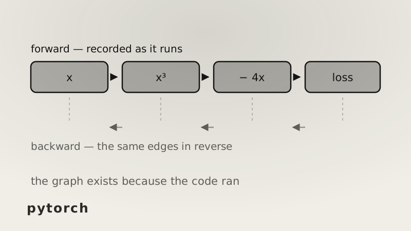
PyTorch builds the computation graph by running your code, which is why ordinary Python control flow works inside a model. The same decision explains its two most common bugs.
PyTorch gives you three things: an array type that runs on a GPU, automatic derivatives, and the layers and optimizers built on top of those two.
The array part is unsurprising — a tensor is a multidimensional grid of numbers with a shape and a device. The derivatives are where the design decision lives.
Derivatives you do not write
Training needs to know, for every parameter, which direction to nudge it. That is a derivative of the loss with respect to that parameter, and for a real model there are billions of them through dozens of composed operations.
Nobody derives those by hand. PyTorch records the operations as they happen and differentiates the record.
x = torch.tensor(2.5, requires_grad=True)
y = x**3 - 4*x
y.backward()
x.grad          # tensor(14.7500)
The derivative of x³ − 4x is 3x² − 4, which at 2.5 is 14.75. Nothing symbolic happened — PyTorch knows the derivative rule for each primitive operation and applied the chain rule backwards through the three it saw.
Built by running
That last phrase is the point. The graph does not exist before the code runs; it is assembled as each operation executes, and it records exactly the operations that actually happened.
Which means ordinary Python works inside a model:
for layer in self.blocks:
    h = layer(h)
    if h.abs().max() > threshold:      # a real branch, on real values
        h = self.rescale(h)
The branch is evaluated with actual numbers, and whichever path was taken is what gets differentiated. A framework that compiled the graph in advance would need that condition expressed in its own special vocabulary, because at compile time there is no value to test.
The same property makes debugging normal. A tensor holds numbers you can print, an exception has a Python stack trace pointing at your line, and a breakpoint stops in the middle of a forward pass. None of that is true of a system where your code only describes a graph that runs later.
The two bugs this design causes
Both follow directly from "the graph is a live object".
Gradients accumulate instead of replacing. Calling backward() adds into .grad rather than overwriting it. Call it twice without clearing and the gradient is 29.50 where the true value is 14.75 — exactly double, and nothing errors. Which is why every training loop starts with optimizer.zero_grad(), and why forgetting it produces a model that trains badly rather than a model that crashes.
This is not an oversight. Accumulation is what makes gradient accumulation over several small batches possible, and what lets two loss terms contribute to the same parameters. The default serves the harder case, and the easy case has to opt out.
Holding a tensor holds the whole graph. A tensor produced by a differentiable operation carries a reference to the operation that made it, which references its inputs, and so on back to the parameters.
So this quietly consumes everything:
total += loss # keeps this batch's entire graph aliveFive hundred batches, each retaining a graph worth a few megabytes, is gigabytes held for a number you wanted to average. The fix is to take the number and drop the graph:
total += loss.item()The same reasoning explains with torch.no_grad() around evaluation. Nothing there needs derivatives, so recording the graph is pure cost — memory and time spent building a structure that will never be read.
Devices
A tensor lives somewhere, and operations require their operands to live in the same place.
device = "cuda" if torch.cuda.is_available() else "cpu"
model.to(device)
batch = batch.to(device)
That is the whole of it, and the explicitness is deliberate. A framework that moved data automatically would hide transfers across a link far slower than either processor's own memory — and a training loop that accidentally copies every batch back and forth spends most of its time on the bus rather than on arithmetic.
Layers, and what they really are
nn.Module is bookkeeping. It tracks which tensors are parameters so an optimizer can find them, holds child modules, and gives you train() and eval() to switch behaviour for layers that differ between the two.
An optimizer is equally plain: given the parameters and their .grad values, apply an update rule. It does not participate in the graph at all — it runs after the backward pass has left gradients behind.
Which leaves the training loop as four lines that say exactly what they do: forward, loss, backward, step.
What to take away
One decision explains most of PyTorch: the graph is created by running your code.
That is why Python control flow, printing and debuggers all work inside a model — and why gradients accumulate, why the graph is freed after backward(), and why keeping a loss tensor around costs you memory. The ergonomics and the footguns come from the same place.