Variational autoencoders
/AI/5 min read
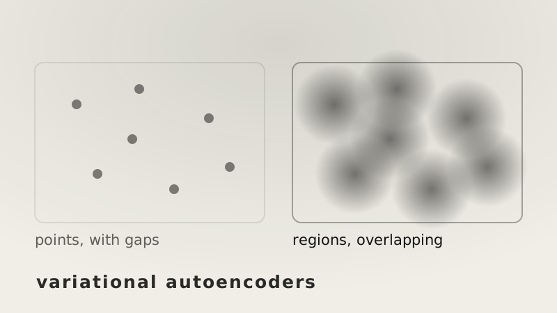
An ordinary autoencoder compresses well and generates nothing, because its latent space is full of holes. A VAE fills the holes by encoding to regions instead of points — and pays for it with a second loss term.
An autoencoder squeezes an input down to a few numbers and then rebuilds it. The encoder compresses, the decoder reconstructs, and training is just "make the output match the input".
It works. And then you try to generate something new by picking a random point in that compressed space and decoding it, and you get noise.
Why the space has holes
Because each input maps to a single point, and nothing ever asked those points to be arranged sensibly.
The encoder places one input here and another over there, with whatever falls between them being territory the decoder has never been trained on. Ask it to decode a point in that territory and it has no reason to produce anything meaningful — it was never shown what belongs there.
The compressed space ends up as scattered islands with empty water between them. Reconstruction works because you only ever decode points the encoder produced. Generation fails because random points are almost never those.
Encoding to a region
The fix is to stop encoding to points.
The encoder outputs two numbers per latent dimension: a centre and a spread . During training a value is sampled from that region and passed to the decoder, so the same input produces a slightly different code every time it is seen.
The decoder therefore has to make the whole region decode to the same thing. And if neighbouring inputs' regions overlap, the space between them is covered by both — no longer empty.
Whether that happens is a matter of arithmetic:
| spread | overlap between regions at 1.5 and 2.0 |
|---|---|
| 0.02 | 0.00% — a gap |
| 0.10 | 1.24% |
| 0.20 | 21.13% |
| 0.40 | 53.20% |
At the two regions do not touch and everything between them is untrained. At they overlap substantially and the space between decodes to something reasonable.
So the spread cannot be left to the encoder, which would happily shrink it to nothing.
Two losses pulling opposite ways
Reconstruction alone wants exactly that: , so the code is precise, and the means pushed far apart, so inputs never get confused. Both give sharper reconstructions and both recreate the hole problem.
The second loss term pushes back. It measures how far each encoded region is from a standard normal — centred at zero, spread of one:
A region at , costs nothing. Shrinking the spread to 0.01 costs 4.11. Pushing the mean out to 3 costs 4.50. Neither of the things reconstruction wants is free.
The trained model sits at the compromise: regions tight enough to reconstruct distinctly, loose enough to overlap. That balance is the whole design, and the ratio between the two terms is the dial that sets it — weight the KL term too heavily and every input encodes to the same blurry region, too lightly and the holes come back.
Sampling without breaking training
There is an obstacle. Training needs gradients, and you cannot differentiate through a random draw — the sampling step sits in the middle of the network and blocks everything behind it.
The way around is to rewrite the draw so the randomness is not in the path:
Mathematically identical — has the same distribution either way. Structurally different: is now an input drawn outside the network, and and reach through a multiplication and an addition, both of which differentiate fine.
The randomness has been moved off the path from the loss to the weights.
Generating
After training, the encoder is set aside. Draw a point from a standard normal, hand it to the decoder, and it produces something new.
That works only because of the KL term. It is what made a standard normal the right thing to sample from — the encoded regions were pulled towards exactly that shape during training, so a random draw from it lands somewhere the decoder understands.
The same property gives interpolation: move gradually from one point to another and the output morphs smoothly, because everything along the path decodes to something.
The cost is sharpness. Averaging over a region means the decoder is trained to produce something acceptable for a whole neighbourhood, and the safe answer for a neighbourhood is a slightly blurred one. That is the recognisable weakness, and it is a direct consequence of the mechanism that fixed the holes.
The short version
- An ordinary autoencoder maps each input to a point, leaving untrained gaps between them.
- Decoding a random point lands in a gap, which is why it cannot generate.
- A VAE encodes to a region — a mean and a spread — and samples from it during training.
- Overlapping regions cover the space between inputs: at σ 0.2 two nearby codes overlap 21%, at σ 0.02 not at all.
- Reconstruction alone would shrink the spread and separate the means, recreating the gaps.
- A KL term charges for both, and is zero exactly at centre 0, spread 1.
- The reparameterisation trick moves the randomness off the gradient path so training still works.
- Generation samples a standard normal — valid only because the KL term shaped the space to match.
- Averaging over regions is also why output tends to be slightly blurry.