Vector databases

An embedding model turns a piece of text into a list of numbers positioned so that things meaning similar things land near each other. Search then becomes geometry: find the stored vectors closest to the query's vector.

A vector database is what makes that lookup fast enough to be useful.

What it holds

Three things per item.

The vector — what similarity is computed against. The original content, because a list of numbers is not something you can show anyone. And metadata: category, date, author, whatever you might want to filter by.

The metadata matters more than it sounds, because most real queries are not pure similarity. "Documents like this one, from this year, that this user may see" is a similarity search with constraints, and whether those constraints are applied before or after the search changes both the cost and the results. Filter first and the search is over a smaller set; search first and you may find that all your nearest neighbours were filtered out.

Measuring closeness

Three measures, and the choice is not arbitrary.

Cosine similarity compares direction only, ignoring length. This is the usual choice for text, because a long document and a short one about the same subject should count as similar, and length otherwise dominates.

Dot product combines direction and magnitude. Identical to cosine when the vectors are normalised to unit length — which most embedding models do, making this the cheaper way to compute the same thing.

Euclidean distance is the straight-line gap. Natural where position genuinely means something rather than just direction.

For normalised vectors these all rank results the same way. The distinction only bites when magnitudes vary.

Why exact search is impossible at scale

Suppose 100 million vectors of 768 dimensions.

Comparing a query against all of them means reading all of them. That is a memory bandwidth problem before it is an arithmetic one:

	bytes read per query	time
brute force, float32	307 GB	6.14 s
brute force, int8	76.8 GB	1.54 s
clustered, examine 0.78%	2.40 GB	48 ms
clustered and compressed to 8 bytes	6.25 MB	0.13 ms

Six seconds a query is not a search product. And note that the two fixes are independent — one reduces how many vectors are examined, the other reduces the bytes per vector — which is why they are almost always used together.

Examining fewer

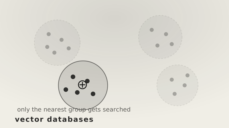
Clustering. Group the vectors and store a centre for each group. At query time, compare against the centres, pick the nearest few groups, and search only those. With 1,024 clusters and 8 probed, that is 0.78% of the data.

Layered graphs. Build a graph connecting each vector to its near neighbours, with sparse upper layers for long jumps and a dense bottom layer for fine steps. A search enters at the top, travels in large hops toward the query's region, then descends for precision. This is the common default, because it holds high recall without needing the data to cluster cleanly.

Both skip most of the data. Both can therefore miss the true nearest neighbour — if it happened to sit in a cluster that was not probed, it is simply not found.

Making each vector smaller

Storing 768 float32 values is 3,072 bytes per vector, and 307 GB for a hundred million.

The blunt approach is fewer bits per number — int8 instead of float32 divides everything by four, and works better than it sounds because embedding comparisons are robust to that much rounding.

The aggressive approach splits each vector into chunks, builds a small codebook of representative chunks, and stores the index of the nearest codebook entry rather than the values. A 768-dimensional vector becomes 8 bytes.

	index size
float32	307 GB
int8	76.8 GB
8-byte codes	0.80 GB

384 times smaller. That is the difference between an index that needs a rack and one that fits in memory on a single machine, which is usually the difference that decides an architecture.

What you give up

All of this is approximate. The measure is recall: of the true ten nearest neighbours, how many were actually returned.

Brute force gives 100% and takes six seconds. Production settings typically sit around 95%, and each configuration knob — clusters probed, graph connectivity, compression level — trades recall for speed.

That trade is usually correct. Nine of the right ten in a millisecond beats all ten in six seconds for nearly every application, especially since the embedding is itself an approximation of meaning — an exact search over approximate coordinates is not exact in any sense the user cares about.

The exception is anywhere a missed match is expensive rather than merely disappointing. Deduplication, compliance checks, anything where a near-duplicate slipping through is the failure — those want the recall pushed high and the cost paid.

The short version

• Store vectors, the original content, and metadata to filter by.
• Cosine for text, dot product when vectors are normalised, Euclidean where position means something.
• Brute force over 100M × 768 float32 vectors reads 307 GB per query — about six seconds.
• Two independent fixes: examine fewer vectors, and shrink each one.
• Clustering or a layered graph cuts what is examined to under 1%.
• Compression takes 3,072 bytes per vector down to 8, and the index from 307 GB to 0.80 GB.
• Together: 0.13 ms instead of 6.14 s.
• The result is approximate. Recall is the dial, ~95% is typical, and that is usually the right call.