Contrastive learning

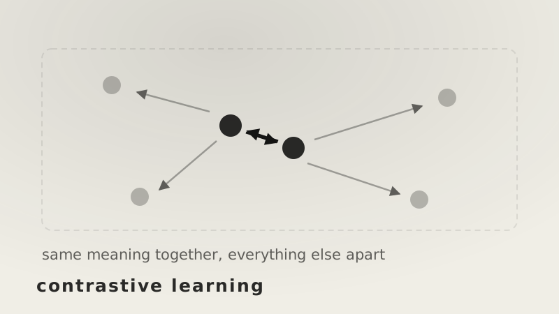
Supervised learning needs labels, and labels are expensive. Contrastive learning gets around that by asking a question the data can answer on its own: which of these things belong together?

Two crops of the same photograph belong together. That photograph and a different one do not. Nobody had to write either fact down.

The setup

Take one item — call it the anchor. Produce a positive: something that should mean the same thing. For an image, that is a different crop, rotation or colour shift of the same picture; for a caption model it is the caption that actually goes with the image; for search it is a passage that genuinely answers the query.

Then take negatives: everything else in the batch.

Push all of them through the encoder, and train so the anchor's embedding is closer to the positive than to any negative. Repeat over enough data and the embedding space arranges itself by meaning, without a single label.

The one rule about augmentation: it has to change appearance while preserving meaning. Crop, flip, recolour — fine. Crop so tightly that the subject is gone and you have taught the model that two unrelated things are the same.

The loss

The one in general use frames it as a multiple-choice question. Given the anchor, which of these candidates is the positive?

$$\mathcal{L} = -\log \frac{\exp(s^{+}/\tau)}{\sum_i \exp(s_i/\tau)}$$

$s$ is a similarity, usually cosine. The numerator is the positive; the denominator sums over the positive and every negative. It is a softmax over candidates, and the loss is just cross-entropy against the correct one.

Which means the difficulty scales with the number of candidates. A model that cannot tell them apart at all scores $\log N$:

candidates	loss floor
8	2.079
256	5.545
1,024	6.931
32,768	10.397

That is why batch size matters so much here in a way it does not elsewhere. The batch is the set of wrong answers, so a bigger batch is a harder exam.

Where the learning actually comes from

Here is the part that is easy to miss. Take an anchor whose positive scores 0.65, against five negatives scoring 0.55, 0.40, 0.35, 0.30 and 0.20.

At a typical temperature of 0.07, this is how the negatives divide up the pressure:

The single hardest negative takes 82.7% of the pressure. The easiest one takes 0.6% — the model has already learned to separate it, so there is nothing left to learn from it.

This is why hard negatives matter more than the number of negatives. A batch of a thousand items where 998 are obviously unrelated is barely more informative than a batch of five. What teaches the model is the candidate it nearly picked.

It is also why some setups mine hard negatives deliberately, and why sampling negatives at random from a large diverse dataset works less well than it looks like it should.

What temperature does

$\tau$ divides every similarity before the softmax, so it controls how sharply the loss distinguishes between candidates:

$\tau$	loss	hardest negative's share
0.01	0.0000	0.0%
0.05	0.1359	11.8%
0.07	0.2546	18.6%
0.10	0.4325	23.9%
1.00	1.5617	19.0%

Very low and the loss collapses to nearly zero — the positive's small lead is exaggerated into certainty, and the model is told it has already succeeded when it has barely separated anything.

Very high and everything blurs together; the loss is large but its gradient no longer distinguishes the near-miss from the obvious miss.

The values in common use sit around 0.05 to 0.1, which is where the hardest negative gets substantial weight without the loss saturating.

The variants

Two views of one item. Augment an image twice, treat the pair as positive, and use every other image in the batch as negatives. Purely self-supervised — no labels anywhere.

A queue of negatives instead of a batch. Keeping a large batch in memory is expensive, so hold a rolling queue of embeddings from recent batches and draw negatives from that. A slowly-updated copy of the encoder keeps the stored embeddings from going stale.

Two modalities. Encode images with one encoder and captions with another, and make the correct image-caption pair the positive while every other pairing in the batch is a negative. This is what puts two different kinds of data into one comparable space.

No negatives at all. A later family drops them entirely, relying on architectural asymmetries — a stop-gradient, a momentum copy, a prediction head — to stop the model taking the shortcut of mapping everything to the same point. Simpler to run, since batch size stops being critical, and less obvious why it works.

The short version

• Learn representations by pulling matching things together and pushing others apart, with no labels required.
• Positives come from augmentation, pairing, or known correspondence; negatives are usually the rest of the batch.
• The loss is cross-entropy over candidates, so its floor is $\log N$ — a bigger batch is a harder question.
• Almost all the gradient comes from the hardest negative: 82.7% from one candidate in the example above.
• Which makes negative quality matter more than negative count.
• Temperature sets how sharply near-misses are distinguished; too low and the loss saturates at nothing.
• Some methods drop negatives entirely and prevent collapse architecturally instead.